Respiratory Illness Patterns in Ottawa
I. Motivation
Respiratory illnesses place a recurring seasonal burden on healthcare systems. Understanding how outbreaks translate into emergency department (ED) visits can help anticipate healthcare demand and identify vulnerable populations.
This project investigates how institutional respiratory outbreaks relate to ED utilization in Ottawa, with a focus on age-specific effects and seasonal dynamics.
This project was prepared as a submission to the R-Ladies Ottawa International Women’s Day Data Challenge (2026).

II. Data Sources
This analysis combines two datasets from Ottawa Public Health:
- Emergency Department Visits: Weekly counts of respiratory-related visits by age group.
- Respiratory Outbreaks: Weekly outbreaks in schools, healthcare institutions, and congregate care settings.
The data allows us to explore how outbreaks affect ED utilization and identify vulnerable populations by age and setting.

This dataset measures healthcare burden and contains weekly counts of emergency department (ED) visits.
The datasets were obtained from Open Ottawa and are publicly available for download:
III. Research questions
We model the relationship between outbreaks and healthcare utilization as:
\[ \text{Outbreaks}_{t-1} \rightarrow \text{Community transmission}_t \rightarrow \text{ED visits}_t \]
Because infections take time to develop into severe symptoms, outbreak counts are lagged by one week.
TipThis project investigates the following questions:
- Do increases in respiratory outbreaks predict increases in emergency visits?
- Are certain age groups more sensitive to outbreaks than others?
- Is the current season above or below historical baseline?
- Do outbreaks in specific settings (schools, healthcare, congregate care) predict increases in respiratory-related ED visits for different age groups?
IV. Data preparation
Datasets were cleaned, aligned by epidemiological week, and merged. Outbreak variables were renamed and aggregated into a total outbreak measure.
library(tidyverse)
library(lubridate)
library(here)

ed <- read.csv(here("data", "All_causes_and_respiratory_related_emergency.csv"), header = TRUE)
outbreaks <- read.csv(here("data", "Respiratory_Outbreaks_(excluding_COVID-19).csv"), header = TRUE)

merged <- ed |>
        left_join(outbreaks, by = c("Epidemiological_Week" = "Start_of_the_Week"))

ed <- ed |>
        mutate(Epidemiological_Week = ymd(Epidemiological_Week))

outbreaks <- outbreaks |>
        mutate(Start_of_the_Week = ymd(Start_of_the_Week))

merged <- merged |>
  rename(
    outbreaks_school =
      Number_of_Respiratory_Outbreaks__Excl__COVID_19__in_Schools__Camps__and_Licensed_Child_Care,
    outbreaks_health =
      Number_of_Respiratory_Outbreaks__Excl__COVID_19__in_Healthcare_Institutions,
    outbreaks_congregate =
      Number_of_Respiratory_Outbreaks__Excl__COVID_19__in_Congregate_Care,

    prev_avg_school =
        Previous_3_Season_Average_of_Respiratory_Outbreaks__Excl__COVID_19__in_Schools__Camps__and_Child_Care,
    prev_avg_health =
        Previous_3_Season_Average_of_Respiratory_Outbreaks__Excl__COVID_19__in_Healthcare_Institutions,
    prev_avg_congregate =
      Previous_3_Season_Average_of_Respiratory_Outbreaks__Excl__COVID_19__in_Congregate_Care,

    pre_covid_school =
      Prior_to_COVID_19_3_Season_Average_of_Respiratory_Outbreaks_in_Schools__Camps__and_Child_Care,
    pre_covid_health =
      Prior_to_COVID_19_3_Season_Average_of_Respiratory_Outbreaks_in_Healthcare_Institutions,
    pre_covid_congregate =
      Prior_to_COVID_19_3_Season_Average_of_Respiratory_Outbreaks_in_Congregate_Care
  )

merged <- merged |>
  mutate(total_outbreaks =
           outbreaks_school + outbreaks_health + outbreaks_congregate)
merged <- merged |>
  mutate(total_outbreaks_prev =
           prev_avg_school + prev_avg_health + prev_avg_congregate)
merged <- merged |>
  mutate(total_outbreaks_pre_covid =
           pre_covid_school + pre_covid_health + pre_covid_congregate)
V. Exploratory analysis
The goal of this section is to assess whether there is evidence of a temporal relationship between respiratory outbreaks and ED visits, and to guide model specification.
Seasonal patterns by age group
Respiratory-related ED visits exhibit strong seasonal patterns across all age groups, with consistent peaks during early winter.
Younger age groups show sharper increases during peak periods, suggesting greater responsiveness to seasonal transmission cycles. However, these differences may also reflect variation in healthcare-seeking behavior or baseline utilization across age groups.
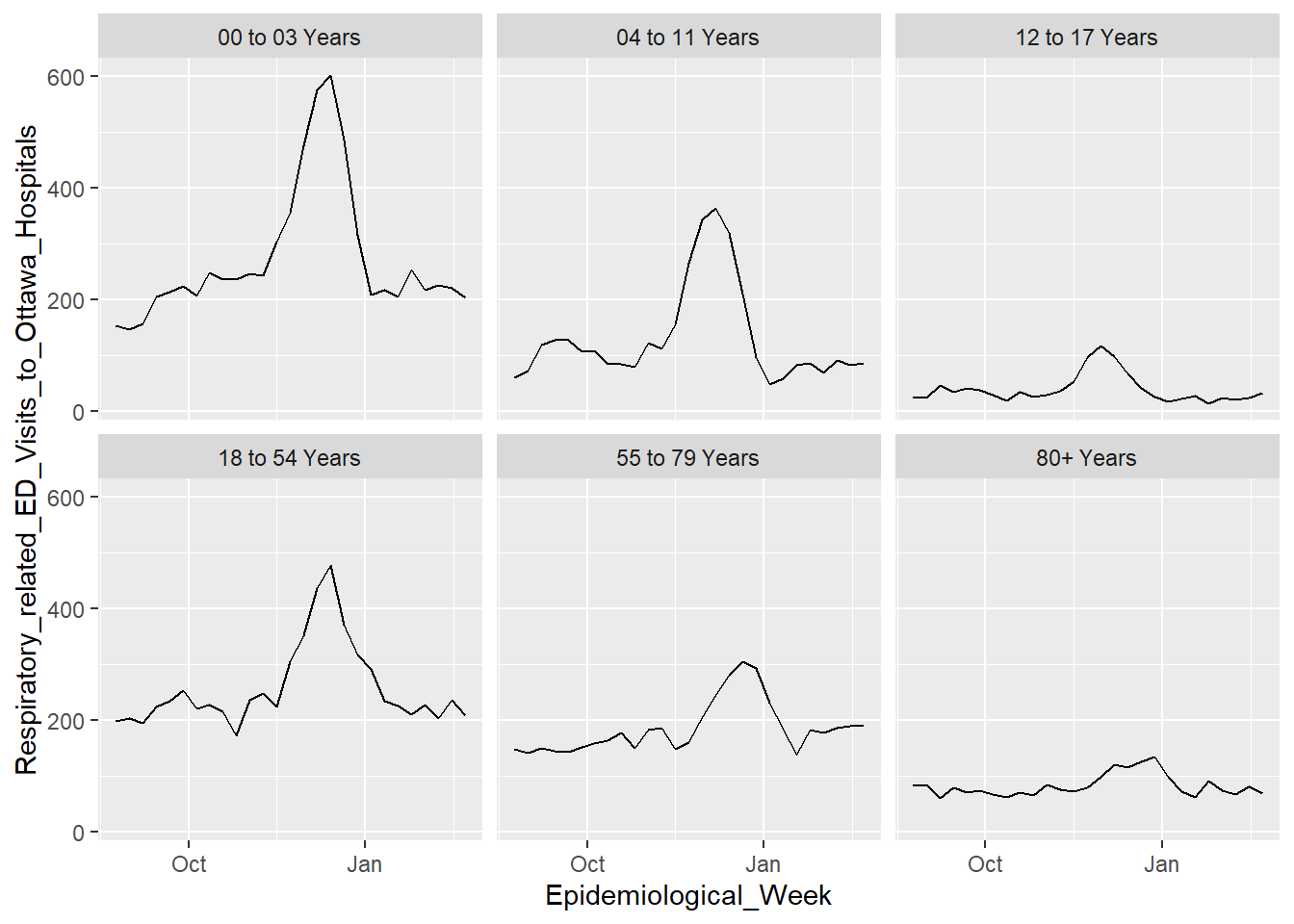
ggplot(merged,
aes(x = Epidemiological_Week,
y = Respiratory_related_ED_Visits_to_Ottawa_Hospitals,
group = Age_Category)) +
geom_line() +
facet_wrap(~Age_Category)
plot_df <- merged |>
mutate(
ed_scaled = scale(Respiratory_related_ED_Visits_to_Ottawa_Hospitals),
outbreaks_scaled = scale(total_outbreaks)
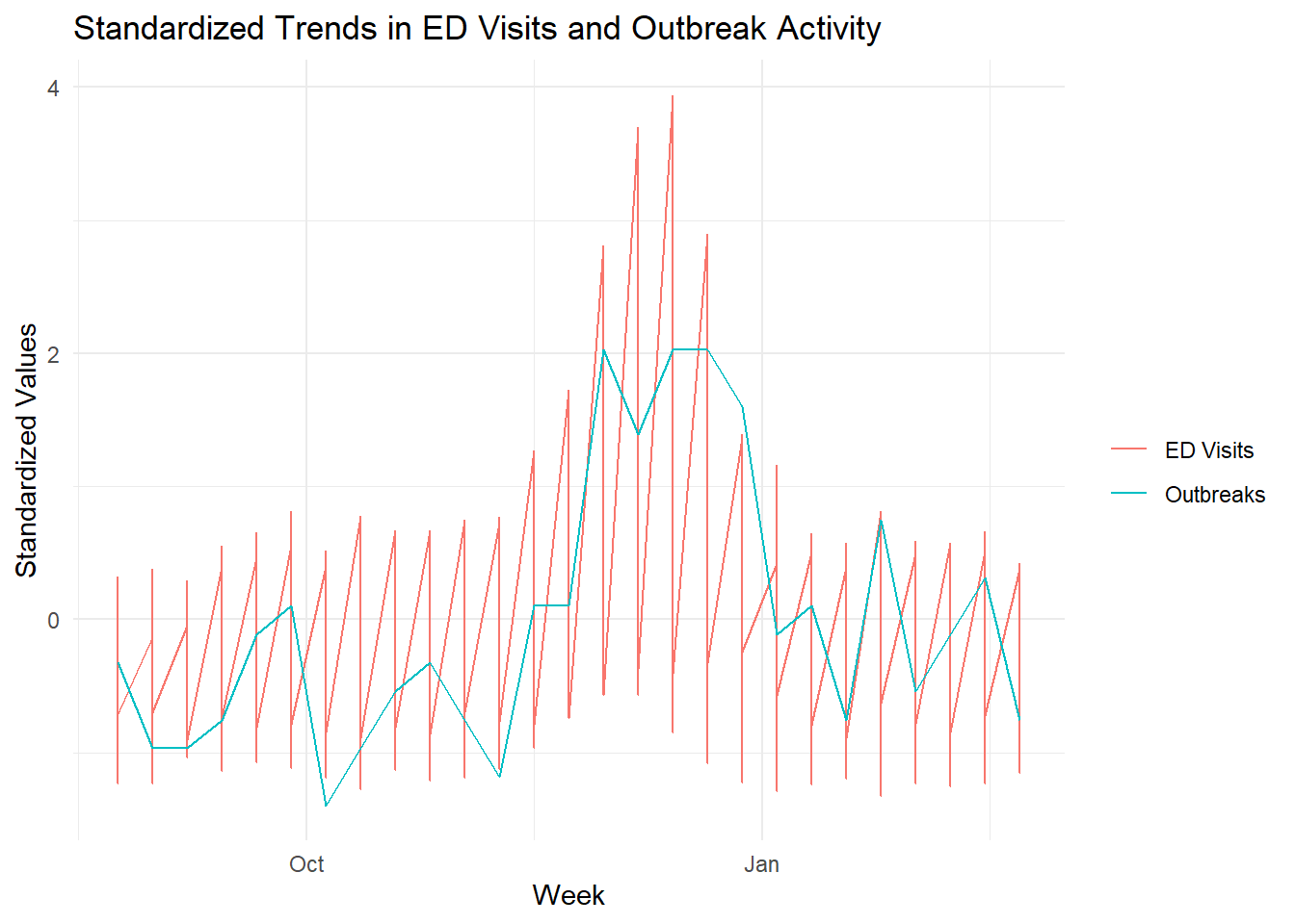
)Alignment between outbreaks and ED Visits
To compare overall trends, both ED visits and outbreak counts are standardized.
Both series display similar seasonal patterns, with increases in outbreak activity aligning closely with rises in ED visits. This suggests a potential temporal relationship between outbreak intensity and healthcare utilization.
plot_df <- merged |>
  mutate(
    ed_scaled = scale(Respiratory_related_ED_Visits_to_Ottawa_Hospitals),
    outbreaks_scaled = scale(total_outbreaks)
  )

ggplot(plot_df, aes(x = Epidemiological_Week)) +
  geom_line(aes(y = ed_scaled, color = "ED Visits")) +
  geom_line(aes(y = outbreaks_scaled, color = "Outbreaks")) +
  labs(
    title = "Standardized Trends in ED Visits and Outbreak Activity",
    y = "Standardized Values",
    x = "Week",
    color = ""
  ) +
  theme_minimal()
Lag structure
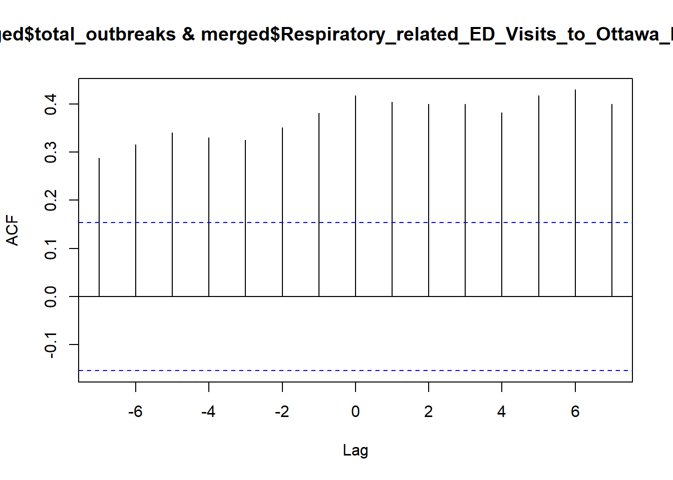
We further examine the timing of this relationship using cross-correlation analysis.
Significant correlations are observed at multiple lags, including 0, 1, and higher-order lags.
From an epidemiological perspective, a short delay between outbreaks and ED visits is expected. Based on this, and for interpretability, we proceed with a one-week lag in subsequent models.
ccf(merged$total_outbreaks,
    merged$Respiratory_related_ED_Visits_to_Ottawa_Hospitals, lag.max = 7)
VI. Lagging for Outbreak Effects
To account for the delay between exposure and healthcare utilization, we introduce a one-week lag on outbreak counts.
This reflects the epidemiological expectation that increases in institutional outbreaks may precede increases in respiratory illness severity requiring emergency care.
\[ \text{ED}_t = \beta_0+\beta_1\text{Outbreaks}_{t-1}+\epsilon \]
Where:
\(\text{ED}_t\) is emergency departmwent visits at week \(t\),
\(\text{Outbreaks}_{t-1}\) is outbreak activity in the previous week
We construct lagged variables for:
Total outbreak activity
and each outbreak setting (school, healthcare, congregate care)
This allows us to compare whether specific settings have distinct temporal effects and whether a single aggregated outbreak measure is sufficient.
VII. Regression Analysis
We model weekly respiratory ED visits as a function of lagged outbreak activity and age group.
To understand how respiratory outbreaks influence emergency department (ED) visits, we evaluate a series of models with increasing complexity.
Our goal is to identify a model that balances:
Interpretability (clear, meaningful effects)
Predictive performance (explains variation in ED visits)
Statistical validity (avoids unnecessary complexity or instability)
Model 1: Baseline Association Model
We begin with a model that includes lagged outbreak counts and age category, but no interaction terms.
This assumes that outbreaks affect all age groups equally.
model1 <- lm(Respiratory_related_ED_Visits_to_Ottawa_Hospitals ~
               lag_school + lag_health + lag_congregate + Age_Category,
              data = analysis_df)
summary(model1)
Call:
lm(formula = Respiratory_related_ED_Visits_to_Ottawa_Hospitals ~
    lag_school + lag_health + lag_congregate + Age_Category,
    data = analysis_df)

Residuals:
     Min       1Q   Median       3Q      Max
-144.737  -32.334   -1.003   21.170  296.731

Coefficients:
                           Estimate Std. Error t value Pr(>|t|)
(Intercept)                 231.558     13.477  17.182  < 2e-16 ***
lag_school                  -19.745     24.736  -0.798    0.426
lag_health                    5.747      1.128   5.097 1.05e-06 ***
lag_congregate               67.435     14.245   4.734 5.13e-06 ***
Age_Category04 to 11 Years -143.462     16.417  -8.739 4.91e-15 ***
Age_Category12 to 17 Years -238.346     16.417 -14.518  < 2e-16 ***
Age_Category18 to 54 Years  -18.462     16.417  -1.125    0.263
Age_Category55 to 79 Years  -91.115     16.417  -5.550 1.30e-07 ***
Age_Category80+ Years      -195.385     16.417 -11.901  < 2e-16 ***
---
Signif. codes:  0 '***' 0.001 '**' 0.01 '*' 0.05 '.' 0.1 ' ' 1

Residual standard error: 59.19 on 147 degrees of freedom
Multiple R-squared:  0.7398,    Adjusted R-squared:  0.7257
F-statistic: 52.25 on 8 and 147 DF,  p-value: < 2.2e-16
TipInterpretation
Lagged healthcare and congregate outbreaks are positively associated with ED visits.
School outbreaks show weak or inconsistent association in this specification.
Age group is a strong predictor of baseline ED utilization.
Younger children (0–3) have the highest baseline ED usage, with all other groups significantly lower
However, this model assumes a constant effect across age groups, which may be unrealistic
Model 2: Interaction Model (Do outbreak effects differ by age?)
We extend the baseline model by allowing outbreak effects to vary across age groups.
This tests whether the association between outbreak activity and ED visits differs by population subgroup.
\[ \text{ED Visits} = \text{(Outbreaks)} \times \text{(Age Category)} \]
model2 <- lm(
  Respiratory_related_ED_Visits_to_Ottawa_Hospitals ~
    (lag_school + lag_health + lag_congregate) * Age_Category,
  data = analysis_df
)

summary(model2)
Call:
lm(formula = Respiratory_related_ED_Visits_to_Ottawa_Hospitals ~
    (lag_school + lag_health + lag_congregate) * Age_Category,
    data = analysis_df)

Residuals:
     Min       1Q   Median       3Q      Max
-181.387  -17.432   -0.073   16.481  268.459

Coefficients:
                                          Estimate Std. Error t value Pr(>|t|)
(Intercept)                                188.537     18.862   9.996  < 2e-16
lag_school                                 -48.923     56.037  -0.873 0.384222
lag_health                                  11.231      2.554   4.397 2.24e-05
lag_congregate                             124.037     32.271   3.844 0.000188
Age_Category04 to 11 Years                 -91.821     26.675  -3.442 0.000773
Age_Category12 to 17 Years                -153.052     26.675  -5.738 6.26e-08
Age_Category18 to 54 Years                  -1.184     26.675  -0.044 0.964663
Age_Category55 to 79 Years                 -55.081     26.675  -2.065 0.040891
Age_Category80+ Years                     -127.503     26.675  -4.780 4.61e-06
lag_school:Age_Category04 to 11 Years       46.359     79.249   0.585 0.559559
lag_school:Age_Category12 to 17 Years       46.047     79.249   0.581 0.562197
lag_school:Age_Category18 to 54 Years       22.141     79.249   0.279 0.780387
lag_school:Age_Category55 to 79 Years       24.396     79.249   0.308 0.758688
lag_school:Age_Category80+ Years            36.125     79.249   0.456 0.649252
lag_health:Age_Category04 to 11 Years       -8.756      3.613  -2.424 0.016711
lag_health:Age_Category12 to 17 Years      -11.833      3.613  -3.275 0.001348
lag_health:Age_Category18 to 54 Years       -1.326      3.613  -0.367 0.714139
lag_health:Age_Category55 to 79 Years       -2.886      3.613  -0.799 0.425816
lag_health:Age_Category80+ Years            -8.104      3.613  -2.243 0.026552
lag_congregate:Age_Category04 to 11 Years   20.512     45.637   0.449 0.653836
lag_congregate:Age_Category12 to 17 Years  -68.956     45.637  -1.511 0.133189
lag_congregate:Age_Category18 to 54 Years  -62.142     45.637  -1.362 0.175632
lag_congregate:Age_Category55 to 79 Years -119.118     45.637  -2.610 0.010098
lag_congregate:Age_Category80+ Years      -109.909     45.637  -2.408 0.017408

(Intercept)                               ***
lag_school
lag_health                                ***
lag_congregate                            ***
Age_Category04 to 11 Years                ***
Age_Category12 to 17 Years                ***
Age_Category18 to 54 Years
Age_Category55 to 79 Years                *
Age_Category80+ Years                     ***
lag_school:Age_Category04 to 11 Years
lag_school:Age_Category12 to 17 Years
lag_school:Age_Category18 to 54 Years
lag_school:Age_Category55 to 79 Years
lag_school:Age_Category80+ Years
lag_health:Age_Category04 to 11 Years     *
lag_health:Age_Category12 to 17 Years     **
lag_health:Age_Category18 to 54 Years
lag_health:Age_Category55 to 79 Years
lag_health:Age_Category80+ Years          *
lag_congregate:Age_Category04 to 11 Years
lag_congregate:Age_Category12 to 17 Years
lag_congregate:Age_Category18 to 54 Years
lag_congregate:Age_Category55 to 79 Years *
lag_congregate:Age_Category80+ Years      *
---
Signif. codes:  0 '***' 0.001 '**' 0.01 '*' 0.05 '.' 0.1 ' ' 1

Residual standard error: 54.74 on 132 degrees of freedom
Multiple R-squared:  0.8002,    Adjusted R-squared:  0.7654
F-statistic: 22.98 on 23 and 132 DF,  p-value: < 2.2e-16
TipInterpretation
The effect of outbreaks is not uniform across age groups.
Congregate care outbreaks show the most consistent association with ED visits.
Healthcare-related outbreaks vary in strength across age groups.
School outbreaks remain weak across most specifications.
Overall, this suggests heterogeneity in how outbreak settings relate to healthcare utilization.
Do interactions improve the model?
We compare the full model (main effects + all interactions) vs the reduced model (main affects only) to see if interaction terms add any useful information.
\[ H_0: \text{Interaction terms do not improve the model fit} \]
\[ H_a:\text{Interaction terms improve model fit} \]
anova(model1, model2)Analysis of Variance Table
Model 1: Respiratory_related_ED_Visits_to_Ottawa_Hospitals ~ lag_school +
lag_health + lag_congregate + Age_Category
Model 2: Respiratory_related_ED_Visits_to_Ottawa_Hospitals ~ (lag_school +
lag_health + lag_congregate) * Age_Category
Res.Df RSS Df Sum of Sq F Pr(>F)
1 147 515057
2 132 395594 15 119463 2.6575 0.0015 **
---
Signif. codes: 0 '***' 0.001 '**' 0.01 '*' 0.05 '.' 0.1 ' ' 1
TipInterpretation
The ANOVA test indicates that adding interaction terms significantly improves model fit (p = 0.00056).
However, the improvement must be weighed against increased model complexity and multicollinearity.
Model 3: Aggregated Outbreak Model (Do we need outbreak categories?)
Because outbreak types are highly correlated, we construct a simplified model using total outbreak activity (to reduce multicollinearity and improve interpretability).
model3 <- lm(
  Respiratory_related_ED_Visits_to_Ottawa_Hospitals ~
    lag_total * Age_Category,
  data = analysis_df
)

summary(model3)
Call:
lm(formula = Respiratory_related_ED_Visits_to_Ottawa_Hospitals ~
    lag_total * Age_Category, data = analysis_df)

Residuals:
    Min      1Q  Median      3Q     Max
-179.63  -23.19   -5.06   18.48  229.38

Coefficients:
                                     Estimate Std. Error t value Pr(>|t|)
(Intercept)                           178.378     20.275   8.798 3.92e-15 ***
lag_total                              15.018      2.491   6.030 1.31e-08 ***
Age_Category04 to 11 Years            -92.022     28.673  -3.209 0.001640 **
Age_Category12 to 17 Years           -146.964     28.673  -5.126 9.39e-07 ***
Age_Category18 to 54 Years              3.984     28.673   0.139 0.889684
Age_Category55 to 79 Years            -45.808     28.673  -1.598 0.112315
Age_Category80+ Years                -118.682     28.673  -4.139 5.91e-05 ***
lag_total:Age_Category04 to 11 Years   -7.731      3.522  -2.195 0.029772 *
lag_total:Age_Category12 to 17 Years  -13.734      3.522  -3.899 0.000147 ***
lag_total:Age_Category18 to 54 Years   -3.373      3.522  -0.958 0.339798
lag_total:Age_Category55 to 79 Years   -6.809      3.522  -1.933 0.055171 .
lag_total:Age_Category80+ Years       -11.528      3.522  -3.273 0.001333 **
---
Signif. codes:  0 '***' 0.001 '**' 0.01 '*' 0.05 '.' 0.1 ' ' 1

Residual standard error: 59.56 on 144 degrees of freedom
Multiple R-squared:  0.742, Adjusted R-squared:  0.7223
F-statistic: 37.65 on 11 and 144 DF,  p-value: < 2.2e-16
TipInterpretation
Total outbreaks are highly significant (p < 0.001)
Age is highly significant (p < 0.001)
Interaction is significant (p = 0.00025)
Overall outbreak intensity strongly associated with ED visits
Age remains a dominant factor
Age groups respond differently to increases in outbreaks
VIII. Model Selection
We evaluate model assumptions and compare competing models to select a final specification.
We first assess standard linear model assumptions.
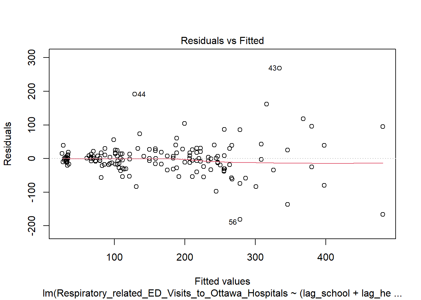
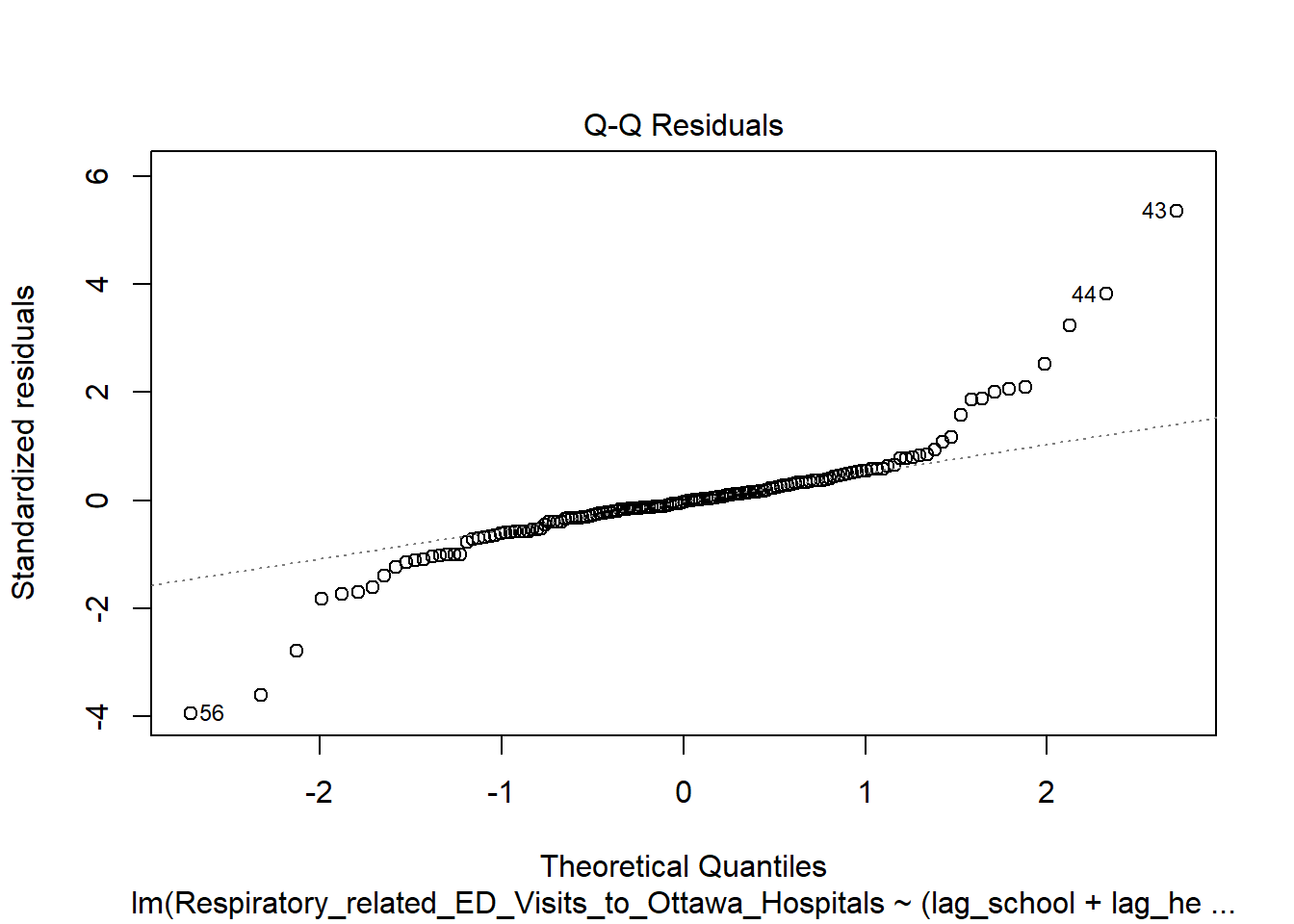
- Slight curvature → mild nonlinearity
- Some spread → mild heteroscedasticity
- Q-Q mostly linear → normality acceptable
We assess multicollinearity using Variance Inflation Factors (VIF).
                                   GVIF Df GVIF^(1/(2*Df))
lag_school                     6.044981  1        2.458654
lag_health                     7.008207  1        2.647302
lag_congregate                 7.056634  1        2.656432
Age_Category                 280.145089  5        1.756865
lag_school:Age_Category        7.334811  5        1.220503
lag_health:Age_Category     1457.780117  5        2.071902
lag_congregate:Age_Category   27.136290  5        1.391089
GVIF Df GVIF^(1/(2*Df))
lag_total 6.0000 1 2.449490
Age_Category 248.2472 5 1.735755
lag_total:Age_Category 660.2284 5 1.914121- Model 2 has high multicollinearity (especially interactions)
- Outbreak types are strongly correlated
- Aggregated model reduces this issue
We compare models using ANOVA, AIC/BIC, and adjusted R².
Analysis of Variance Table

Model 1: Respiratory_related_ED_Visits_to_Ottawa_Hospitals ~ lag_total *
    Age_Category
Model 2: Respiratory_related_ED_Visits_to_Ottawa_Hospitals ~ (lag_school +
    lag_health + lag_congregate) * Age_Category
  Res.Df    RSS Df Sum of Sq      F    Pr(>F)
1    144 510812
2    132 395594 12    115219 3.2038 0.0004715 ***
---
Signif. codes:  0 '***' 0.001 '**' 0.01 '*' 0.05 '.' 0.1 ' ' 1
[1] 0.7222733[1] 0.7653644 df AIC
model2 25 1715.482
model3 13 1731.358 df BIC
model2 25 1791.728
model3 13 1771.006Fit improvement is small / marginal
Barely statistically significant at 5%
R² difference is tiny
We examine influential observations using Cook’s distance and leverage plots.
plot(model2, which = 4) # Cook's distance model2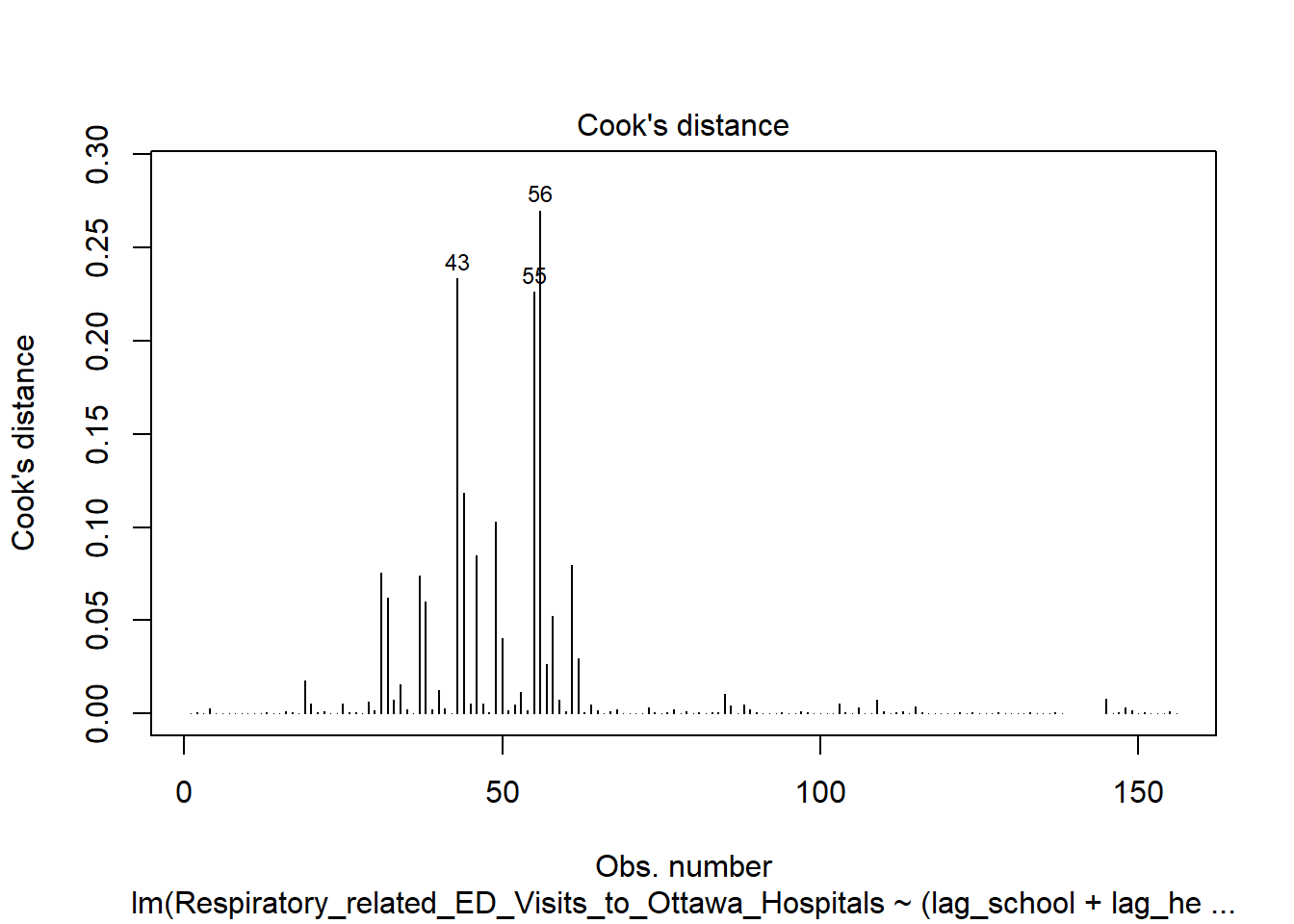
plot(model3, which = 4) # Cook's distance model3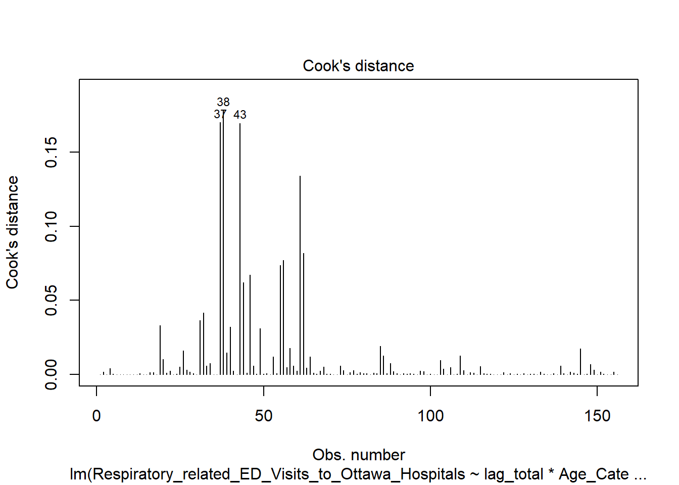
plot(model2, which = 5) # Residuals vs leverage model2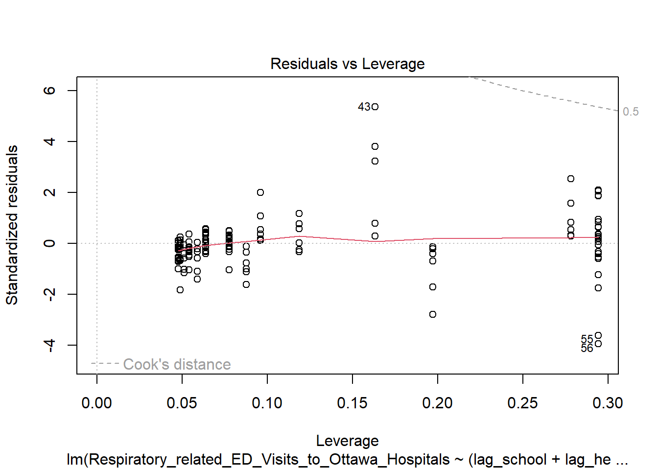
plot(model3, which = 5) # Residuals vs leverage model3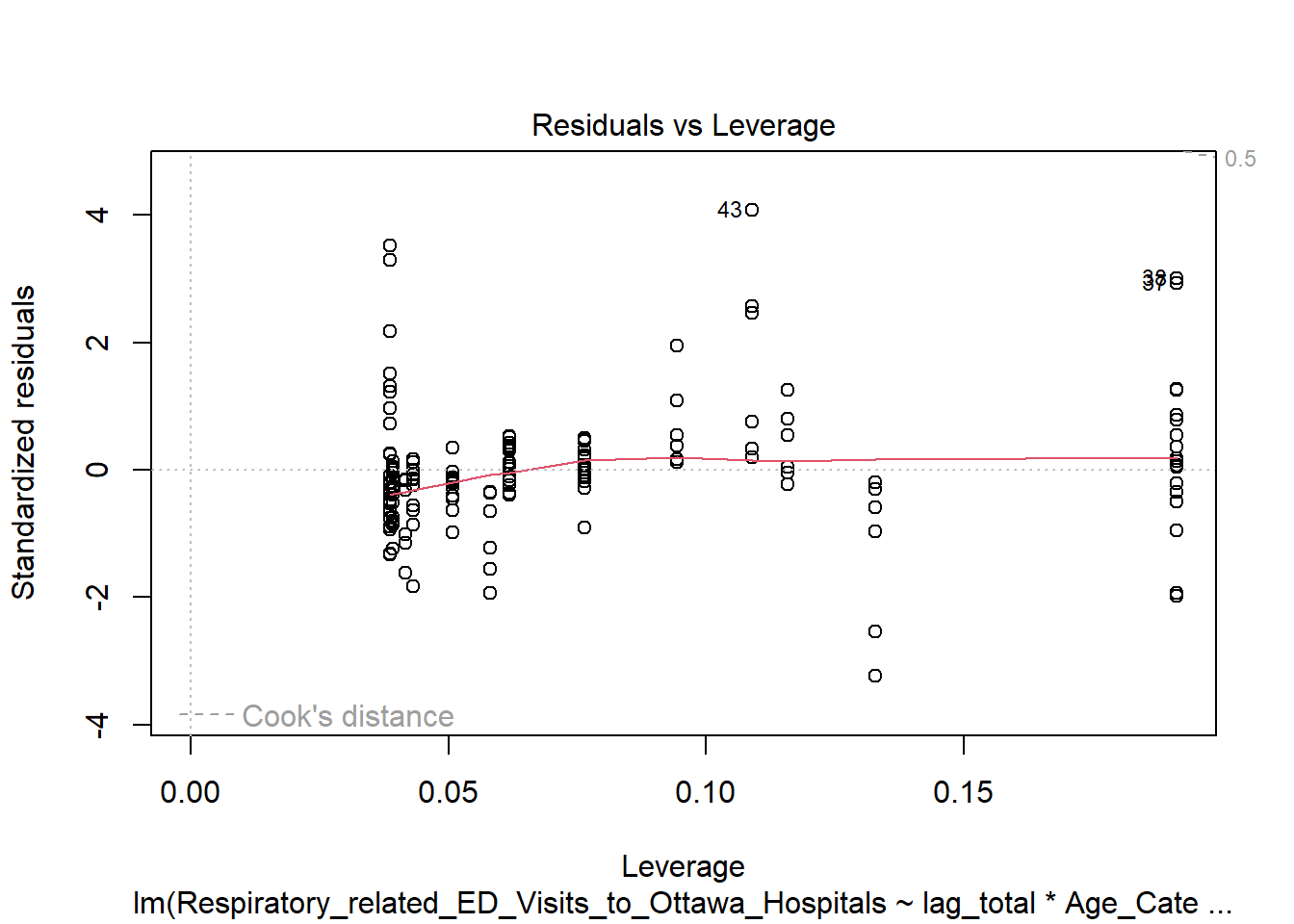
A few influential points exist
More complex model is more sensitive to them
Final model selection
TipInterpretation
We consider three models:
Model 1: main effects only
Model 2: outbreak-by-age interactions (by setting)
Model 3: total outbreaks with age interaction
While Model 2 achieves the best fit, it suffers from:
high multicollinearity
increased sensitivity to influential observations
reduced interpretability
Model 3 achieves comparable explanatory power while remaining:
more parsimonious
more stable
easier to interpret
Final Model:
We select Model 3.
\(\text{ED_visits}_t=\beta_0+\beta1\text{Outbreaks}{t-1}+\beta_2\text{Age}+\beta3 \text{outbreaks}{t-1}\times \text{Age}+\epsilon_t\)
IX. Interpreting the Final Model
Age-Specific Effects of Outbreaks
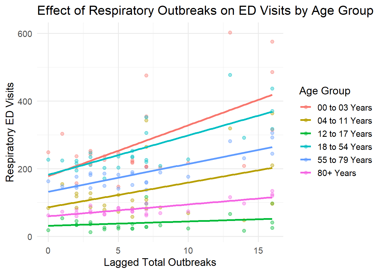
The slope of each line represents how strongly ED visits respond to increases in outbreak activity. Younger age groups show steeper slopes, indicating higher sensitivity to outbreaks, while older groups exhibit flatter responses.
The relationship between lagged outbreak activity and ED visits varies substantially across age groups.
ED visits increase as outbreak activity rises across all groups
However, the magnitude of this increase differs significantly by age
Younger age groups exhibit a much stronger response to increases in outbreak activity, while older groups show more moderate changes. This pattern reflects the interaction between outbreak intensity and age group included in the model.
library(ggplot2)

ggplot(analysis_df,
       aes(x = lag_total,
           y = Respiratory_related_ED_Visits_to_Ottawa_Hospitals,
           color = Age_Category)) +
  geom_point(alpha = 0.4) +
  geom_smooth(method = "lm", se = FALSE, size = 1.2) +
  labs(
    title = "Effect of Respiratory Outbreaks on ED Visits by Age Group",
    x = "Lagged Total Outbreaks",
    y = "Respiratory ED Visits",
    color = "Age Group"
  ) +
  theme_minimal(base_size = 14)
Effect sizes
We interpret the interaction model by computing age-specific effects of outbreak activity (see code tab).
Baseline group (0–3 years): A one-unit increase in outbreaks is associated with approximately 15 additional ED visits.
Teenagers (12–17 years): The same increase is associated with only ~1–2 additional visits
This indicates that younger children are substantially more sensitive to changes in outbreak activity.
library(broom)
library(dplyr)

tidy(model3) |>
  filter(term == "lag_total" | grepl("lag_total:Age_Category", term))
# A tibble: 6 × 5
term estimate std.error statistic p.value
<chr> <dbl> <dbl> <dbl> <dbl>
1 lag_total 15.0 2.49 6.03 0.0000000131
2 lag_total:Age_Category04 to 11 Years -7.73 3.52 -2.19 0.0298
3 lag_total:Age_Category12 to 17 Years -13.7 3.52 -3.90 0.000147
4 lag_total:Age_Category18 to 54 Years -3.37 3.52 -0.958 0.340
5 lag_total:Age_Category55 to 79 Years -6.81 3.52 -1.93 0.0552
6 lag_total:Age_Category80+ Years -11.5 3.52 -3.27 0.00133 coef(model3) (Intercept) lag_total
178.377833 15.018360
Age_Category04 to 11 Years Age_Category12 to 17 Years
-92.021656 -146.963952
Age_Category18 to 54 Years Age_Category55 to 79 Years
3.984061 -45.808461
Age_Category80+ Years lag_total:Age_Category04 to 11 Years
-118.681687 -7.730849
lag_total:Age_Category12 to 17 Years lag_total:Age_Category18 to 54 Years
-13.733741 -3.373327
lag_total:Age_Category55 to 79 Years lag_total:Age_Category80+ Years
-6.809133 -11.527608 # baseline (00–03)
base_effect <- coef(model3)["lag_total"]
# example: 12–17
teen_effect <- base_effect + coef(model3)["lag_total:Age_Category12 to 17 Years"]
base_effectlag_total
15.01836 teen_effectlag_total
1.284619 Scenario comparison
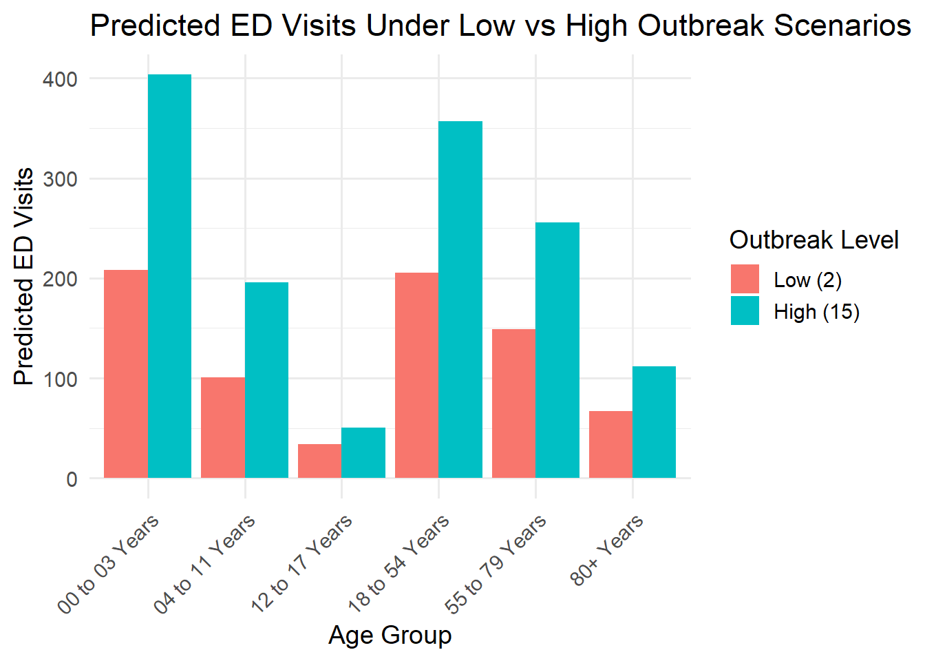
To illustrate the practical impact of outbreak variation, we compare predicted ED visits under two scenarios:
- Low outbreak activity (2 outbreaks/week)
- High outbreak activity (15 outbreaks/week)
Results show:
ED visits among children aged 0–3 increase from ~208 to ~404\
Among teenagers, visits increase only from ~34 to ~51
This demonstrates that increases in outbreak activity disproportionately affect younger populations, placing greater strain on pediatric emergency services.
| Predicted Respiratory ED Visits by Age Group | ||
| Comparison under low vs high outbreak scenarios | ||
| Outbreak Level | Age Group | Predicted ED Visits |
|---|---|---|
| Low (2 outbreaks) | 00 to 03 Years | 208 |
| Low (2 outbreaks) | 04 to 11 Years | 101 |
| Low (2 outbreaks) | 12 to 17 Years | 34 |
| Low (2 outbreaks) | 18 to 54 Years | 206 |
| Low (2 outbreaks) | 55 to 79 Years | 149 |
| Low (2 outbreaks) | 80+ Years | 67 |
| High (15 outbreaks) | 00 to 03 Years | 404 |
| High (15 outbreaks) | 04 to 11 Years | 196 |
| High (15 outbreaks) | 12 to 17 Years | 51 |
| High (15 outbreaks) | 18 to 54 Years | 357 |
| High (15 outbreaks) | 55 to 79 Years | 256 |
| High (15 outbreaks) | 80+ Years | 112 |
library(tidyr)

scenario_df <- expand_grid(
  lag_total = c(2, 15),  # low vs high outbreaks
  Age_Category = unique(analysis_df$Age_Category)
)

library(gt)

scenario_df <- expand_grid(
  lag_total = c(2, 15),  # low vs high outbreaks
  Age_Category = unique(analysis_df$Age_Category)
)

scenario_df$predicted_ED <- predict(model3, newdata = scenario_df)

# Pretty table
scenario_df %>%
  mutate(
    lag_total = ifelse(lag_total == 2, "Low (2 outbreaks)", "High (15 outbreaks)")
  ) %>%
X. Key Findings
TipKey Findings
1. Lagged institutional respiratory outbreaks are positively associated with ED visits.
2. Age group is the strongest determinant of baseline ED utilization.
3. The relationship between outbreaks and ED visits varies across age groups, with young children showing the strongest sensitivity.
4. Disaggregating outbreak settings provides limited additional explanatory value beyond total outbreak activity.
XI. Public Health Implications
This analysis highlights clear age-specific differences in how respiratory outbreak activity relates to emergency department utilization.
Young children (0–3 years) show the strongest response to increases in outbreak activity
Older age groups exhibit more moderate changes
These findings suggest that periods of elevated outbreak activity may place disproportionate strain on pediatric emergency services.
From a planning perspective, monitoring outbreak trends could support:
Early warning systems for increased pediatric ED demand
Resource allocation, particularly staffing and capacity in pediatric care
Targeted interventions in high-risk settings such as congregate care and healthcare institutions
While this analysis is not causal, the consistent temporal relationship between outbreaks and ED visits indicates that outbreak surveillance data may be a valuable input for short-term healthcare planning.
Future work could extend this analysis using count-based time series models (e.g., Poisson or negative binomial regression) to better account for the distributional properties of ED visits.
XII. Limitations
WarningLimitations
This is an observational time-series analysis; causal inference is not possible.
ED visits are count data, and linear regression may not fully capture distributional properties.
Outbreak reporting may be subject to underreporting or reporting delays.
Aggregating outbreak types assumes equal weighting across settings.
Limited time span restricts the complexity of models that can be reliably estimated, increasing risk of overfitting in highly parameterized specifications.
References
Grus, J. (2019). Data Science from scratch: First principles with python. O’Reilly.
Coghlan, A. Using R for Time Series Analysis - Time Series 0.2 documentation. (n.d.). https://a-little-book-of-r-for-time-series.readthedocs.io/en/latest/src/timeseries.html
Pelletier, H. (2025, February 3). How to: Forecast time series using lags. Towards Data Science. https://towardsdatascience.com/how-to-forecast-time-series-using-lags-5876e3f7f473/